Euler Examples

Search

2-Body Problem

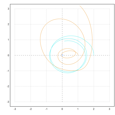
We start with two bodies in space. The function test3body uses an adaptive Runge method to solve the Newtonian equations for the movements of bodies under gravitation.

3-body Documentation

>load 3body;

In the first example, we take two bodies with equal weight, starting with equals speed. The initial positions and speed vectors are

The time interval is one second, and this interval is subdivided into n=100 subintervals by default.

Euler animates the movement of the planets. To save time, the animation is very coarse.

>test2body([-2,0, 2,0, 0,-0.3, 0,0.3],tmax=30):

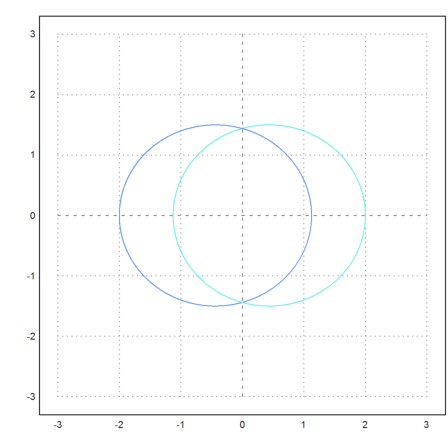
The next example has two different masses. For a smoother animation, we take a time interval of 0.1.

>test2body([0,0, 2,0, 0,-0.2, 0,2],m1=10,m2=1,tmax=5,h=0.1):

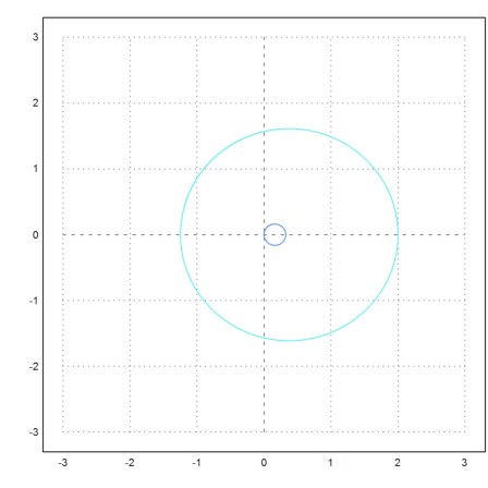
The display can be centered at the first mass. We change the initial speed of the second mass a bit.

>test2body([0,0, 2,0, 0,0, 0,1],m1=10,m2=1,tmax=5,>fixed):

3-Body Problem

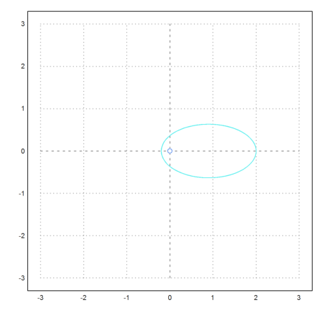
With three bodies, the movements get chaotic.

>test3body([-2,0, 2,0, 0,2, 0.1,-0.2, -0.2,0.2, 0.1,0],n=100):

One body left definition area!

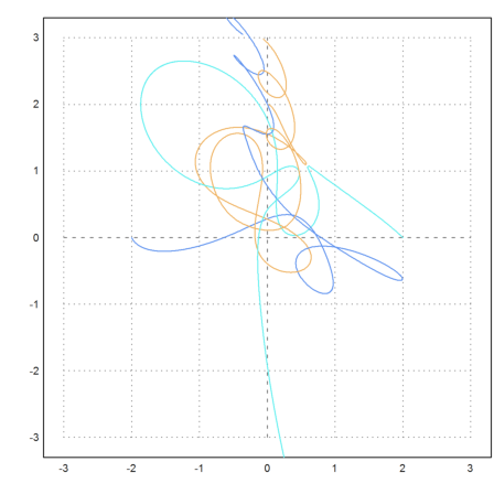
The accuracy is critical here, since the bodies get very close to each other. If you like try n=1000. Then the behaviour does not change much, so we assume that the computation is accurate.

The next example has two starts of mass 1 and 2, and a plante of mass 0.1. The planet will run around the larger star until the smaller one catches the planet for a short time.

>test3body([0,0, 2,0, 1,0, 0,0, 0,1.3, 0,1.2], ...
   m1=2,m2=1,m3=0.1,>fixed,tmax=50):

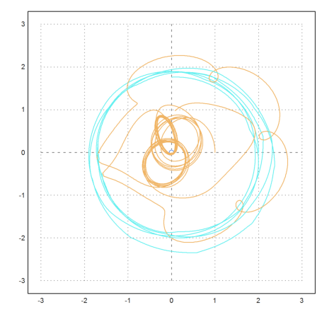
With slightly different initial conditions the small planet gets kicked out of the system very soon.

>test3body([0,0, 2,0, 1,0, 0,0, 0,1, 0,0.5], ...
   m1=2,m2=1,m3=0.1,>fixed,tmax=10):

Examples